

Table of Contents
Short-term demand forecasting predicts how much of each product you will sell over the next few days to roughly three months, so you can decide what to reorder, where to position inventory, and how much warehouse labor to schedule. It differs from long-range planning because the decisions it drives are immediate and hard to reverse once a reorder window closes. For most growing brands, the right approach is not the most sophisticated model available. It is the method that fits your demand patterns and your data, and that connects directly to the operation acting on it.
Stable, high-volume SKUs often forecast well with straightforward averages, while SKUs affected by promotions, multiple sales channels, or shifting seasonality need models that can weigh more inputs at once. Either way, a forecast only creates value when it changes what happens in the warehouse. That is why Cart.com builds forecasting into the same platform that runs inventory, order management, and fulfillment across its nationwide network, so the forecast and the operation work from the same data.
Why short-term forecasting matters to operations teams
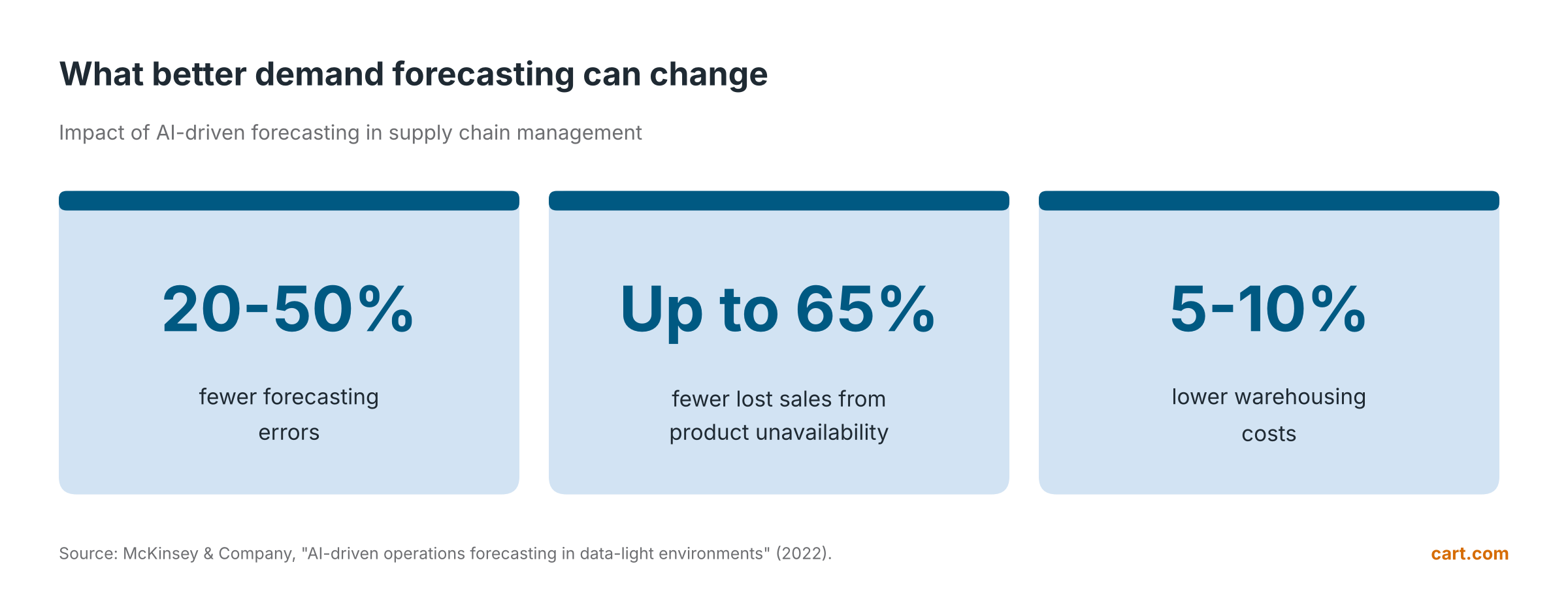
Annual plans set the budget, but short-term forecasts decide whether the right units are on the shelf next week. When those forecasts miss, the cost lands directly on operations in the form of stockouts, rush freight, excess storage, and markdowns. Across retail, the combined cost of overstocks and out-of-stocks reached an estimated $1.7 trillion a year, or 6.2% of global retail sales, according to IHL Group's 2026 Inventory Distortion Study. Better forecasting can close a meaningful share of that gap. McKinsey found that applying AI-driven forecasting to supply chain management can reduce forecasting errors by 20 to 50 percent, which can translate into up to 65 percent fewer lost sales and product unavailability, along with warehousing cost reductions of 5 to 10 percent.
The three main approaches, in plain terms
Forecasting methods fall into three broad tiers. You do not need to know how each one works under the hood to choose well. You need to know what each one requires from your business and where it tends to break down.
| Approach | What it needs from you | Where it fits best | Where it struggles |
|---|---|---|---|
| Simple averages and rules | A few months of sales history and a spreadsheet | Stable, high-volume SKUs with steady demand | Promotions, new products, and sudden demand shifts |
| Statistical seasonal models | Roughly two years of consistent history and some analyst support | Products with predictable trends and seasonal peaks | Many SKUs across channels, and events that break the seasonal pattern |
| Machine learning models | Large, connected data sets spanning sales, channels, and marketing activity | Large catalogs, multichannel selling, and promotion-heavy calendars | Thin or disconnected data, and teams without the resources to build and maintain models |
Simple averages and rules
The simplest approach forecasts next week's demand from the average of recent weeks, sometimes weighting the latest results more heavily. It is cheap, transparent, and easy for any planner to maintain. For a core SKU that sells at a steady rate through one channel, it is often good enough. Its weakness is that it only looks backward, so it reacts to a promotion, a viral moment, or a new wholesale order after the fact rather than before.
Statistical seasonal models
Statistical models identify trend and seasonality in your history and project them forward. They handle predictable patterns well, such as a skincare line that climbs every November or a supplement that spikes each January. They typically need about two full years of consistent data to learn a seasonal cycle reliably, and they take analyst time to tune. They also assume the future will look like the past, which becomes a problem when your channel mix or marketing calendar changes quickly.
Machine learning models
Machine learning models can weigh many inputs at once, including channel-level sales, seasonality, current site performance, and planned campaigns. That makes them well suited to brands selling across DTC, marketplaces, and wholesale, where each channel grows at a different pace. The tradeoff is that they need a large volume of clean, connected data, plus the engineering resources to build and maintain them. For most mid-market brands, that investment is hard to justify in house, which is why more operations leaders are choosing a fulfillment partner that already runs AI forecasting on top of its own inventory and order data.
Is AI demand forecasting always more accurate than simpler methods?
No. Machine learning models tend to outperform simpler methods when demand is influenced by many factors at once and the business has large, clean, connected data sets. For stable products with limited history, a simple average or seasonal model can perform just as well at a fraction of the cost. The best results usually come from matching the method to each product's demand pattern rather than applying one model to the whole catalog.
Your data matters more than your model
The most common reason a forecast fails is not the method. It is the data feeding it. Before choosing an approach, it is worth assessing five things honestly. The first is completeness, meaning whether you have unbroken sales history for each SKU without gaps from system migrations or stockouts that hid true demand. The second is consistency, meaning whether product IDs, units, and channel names match across Shopify, Amazon, wholesale, and your warehouse system. The third is timeliness, meaning how quickly sales and inventory data reach the people and tools making decisions. The fourth is channel coverage, meaning whether every place you sell feeds the same data set. The fifth is context, meaning whether planned promotions, launches, and price changes are recorded somewhere a forecast can use them.
Most brands struggle with these not because of poor discipline, but because their sales channels, inventory, and warehouse run on separate systems. When orders, inventory, and fulfillment already live on one platform, most of the data readiness problem is solved before forecasting begins.
What data do you need for short-term demand forecasting?
At minimum, you need SKU-level sales history by channel, current inventory positions across every location, and supplier lead times. Accuracy improves further when the forecast also includes marketing activity, seasonal patterns, and current ecommerce performance, and when all of this data updates in real time rather than through weekly exports.
How Cart.com connects forecasting to fulfillment
Most forecasting tools stop at a number. Cart.com is built so the forecast flows directly into the decisions that follow it, because forecasting, order management, inventory, and warehouse operations all run on one platform supporting thousands of brands and more than 80 million orders a year across 14 fulfillment and distribution centers.
Forecasts built on more than sales history
Cart.com's AI forecasts future demand at the SKU and sales-channel level using a wide range of data that a spreadsheet forecast rarely captures, including omnichannel marketing and sales history, seasonal patterns, and current ecommerce performance. For a brand selling through its own site, Amazon, and wholesale accounts, that means each channel is forecast on its own trajectory rather than blended into a single average.
From forecast to reorder and placement decisions
A forecast is only useful if it tells you what to do next. Demand AI helps brands determine how much inventory to reorder and where it should be distributed, and it surfaces predictive insights that inform replenishment timing, inventory positioning, and capacity planning. Because inventory syncs across every channel and location in real time, those recommendations are based on what is actually on hand, not last week's export.
Visibility your team can act on
Operations teams need to see the numbers behind a recommendation before they trust it. Cart.com's platform includes 194 built-in reports covering inventory, labor, shipping, orders, and financial performance, so planners can trace a reorder suggestion back to the data that produced it and adjust with confidence.
What this looks like in practice
Tea Collection, a children's apparel brand that has worked with Cart.com since 2012, partnered with Cart.com to assess inventory performance and identify styles with limited future sales potential. Together they flagged hundreds of unproductive and aged SKUs, freeing working capital and aligning stock with actual customer demand. The result was a 32% reduction in reserve storage space and a 75% drop in reserve pallets, from 800 to 200. Read the full Tea Collection case study.
For a closer look at how this applies to the busiest weeks of the year, see our guide to AI demand forecasting for peak season.
What to ask any 3PL about forecasting
Whether or not you choose Cart.com, these questions will show you how seriously a fulfillment partner treats forecasting. Ask whether its forecasting runs on the same platform as its inventory and order management, or whether it depends on exports between disconnected systems. Ask whether inventory syncs across every channel and location in real time, since a forecast built on stale counts will steer reorders in the wrong direction. Ask how forecasts turn into action, including reorder quantities, inventory placement across fulfillment centers, and labor planning. Finally, ask what reporting you will have access to, so your team can see the numbers behind each recommendation rather than taking them on faith.
Frequently asked questions
What is short-term demand forecasting?
Short-term demand forecasting predicts product demand over the next few days to about three months. Brands use it to decide reorder quantities, where to position inventory, and how much warehouse labor to schedule, decisions that are difficult to reverse once lead times pass.
How is short-term forecasting different from long-term forecasting?
Long-term forecasting supports annual budgets, capacity investments, and supplier contracts over a horizon of a year or more. Short-term forecasting drives weekly operational decisions and relies more heavily on recent sales, current inventory, and upcoming promotions.
Which forecasting method should a growing ecommerce brand use?
Most brands benefit from a mix. Simple averages work for stable, high-volume SKUs, seasonal models suit products with predictable peaks, and machine learning models add the most value for large, multichannel catalogs with frequent promotions. Data quality should guide the choice as much as model sophistication.
How much does better demand forecasting reduce costs?
McKinsey found that AI-driven forecasting can reduce forecasting errors by 20 to 50 percent in supply chain settings, which can cut lost sales and product unavailability by up to 65 percent and lower warehousing costs by 5 to 10 percent. Actual results depend on demand volatility, data quality, and how quickly forecasts are acted on.
Should a brand build forecasting in house or rely on its 3PL?
Building advanced forecasting in house requires data engineering, analyst time, and ongoing model maintenance. Many mid-market brands get better results using a 3PL whose forecasting runs on the same platform as its inventory and order management, because the forecast connects directly to replenishment and warehouse planning.
Does Cart.com offer demand forecasting?
Yes. Cart.com's Demand AI forecasts demand at the SKU and sales-channel level using omnichannel sales and marketing history, seasonal patterns, and current ecommerce performance. It runs on the same platform as Cart.com's order management, inventory, and fulfillment operations, so forecasts inform reorder, placement, and capacity decisions directly.
If your team is spending more time reconciling inventory data than acting on it, Cart.com can help. See how Cart.com's fulfillment software and data platform connects forecasting, inventory, and fulfillment in one place, or talk with a fulfillment specialist about building a forecast your warehouse can actually act on.
Related reading: How AI Demand Forecasting Gets Brands Ready for Peak Season Before It Hits, How AI and predictive inventory forecasting are changing the math for fashion brands, Peak season fulfillment planning for fashion brands: a practical capacity guide